Linear Model Predictive Control
Introduction
Model Predictive Control (MPC) is a modern control strategy known for its capacity to provide optimized responses while accounting for state and input constraints of the system. This introduction only provides a glimpse of what MPC is and can do. In fact, MPC is a solid and large research field on its own.
In the core idea of MPC is the fact that a model of the dynamic system (the vehicle in our case) is used to predict the future evolution of the state trajectories in order to optimize the control signal and account for possible violation of the state trajectories while bounding the input to the admissible set of values. The concept is shown in Figure 1.
In the core idea of MPC is the fact that a model of the dynamic system (the vehicle in our case) is used to predict the future evolution of the state trajectories in order to optimize the control signal and account for possible violation of the state trajectories while bounding the input to the admissible set of values. The concept is shown in Figure 1.
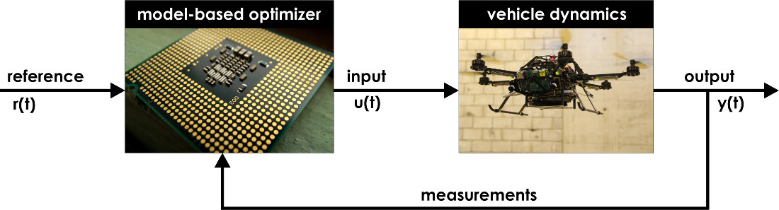
Figure 1: The basic concept of model predictive control as a model-based and optimization-based solution.
Receding Horizon Strategies
Model Predictive Control relies on the concept of receding horizon optimal control derivation. According to this approach, at time t we solve to find the optimal control sequence over a finite future horizon of N steps. The relevant formulation is shown below:
Based on the concept of receding horizon, we derive the optimal sequence over N steps but we only apply its first element - the first optimal control move-action u*(t). At time t+1, we get new measurements/state estimates and repeat the optimization. Essentially, we exploit feedback to update the optimization over the time horizon selected to predict the future evolution of the system outputs.
To understand the concept of receding horizon control, one can consider the analogy of a driver steering a car. Within that analogy:
- Prediction model is what describes how the vehicle is expected to move on the map.
- System Constraints is the set of rules to drive on roads, respect one-ways, don't exceed mechanical capacities of the vehicle.
- Disturbances are the driver's innattention and other reasons for uncontrolled deviation from the desired trajectory.
- Set point is the desired location.
- Cost Function may be the goal of minimum time, minimum distance etc.
Deriving a Good Model for Model Predictive Control
MPC relies on the provided model for its computations. In fact, the model selection has a major role regarding the computational complexity of the algorithm, its theoretical properties (e.g. stability). At the same time, the selected objective and imposed constraints also influence and define these properties.
A good model for MPC is a model that is descriptive enough, captures the dominant and important dynamics of the system but also remains simple enough such that it allows the optimization problem to be tractable and solvable in real-time. Finding a good balance between these two requirements is a balance. A good model is simple as possible, but not simpler.
Therefore, the following questions should be answered before deriving a model to be used with Model Predictive Control methods:
- Should -for control purposes- the system be captured with Nonlinear, Linear or Hybrid dynamics?
- What is the required -for control purposes- order of the system?
- Can we decouple the system? What assumptions are required? Are they reasonable?
Linear MPC Tracking Problem
Considering a system captured using the linear dynamics:
The Optimal Constrained Control Problem of Linear MPC Reference Tracking takes the form:

where:
This Convex Quadratic Program (QP) can be re-written in the more general form:
And the derivation of its solutions can be accomplished using modern methods for Convex Optimization.
Design and Implementation of a Linear MPC
Design, implementation and efficient execution of model predictive control is a very challenging problem that requires deep understanding of optimization methods and strong coding skills. However, the great success of the method lead to the fact that one can use advanced software tools to achieve this goal quite seamlessly. Although deep understanding is always beneficial, implementation of a single MPC may be nothing more than writing a very brief abstract program.
An excellent tool is the "CVXGEN: Code Generation for Convex Optimization". CVXGEN generates fast custom code for small, QP-representable convex optimization problems, using an online interface with no software installation. With minimal effort, turn a mathematical problem description into a high speed solve.
As can be found in the relevant example "Example: Model Predictive Control (MPC)", the following CVX code is enough to produce auto-generated C-code for a Linear MPC:
dimensions
  m = 2  # inputs.
  n = 5  # states.
  T = 10  # horizon.
end

parameters
  A (n,n)  # dynamics matrix.
  B (n,m)  # transfer matrix.
  Q (n,n) psd  # state cost.
  Q_final (n,n) psd  # final state cost.
  R (m,m) psd  # input cost.
  x[0] (n)  # initial state.
  u_max nonnegative  # amplitude limit.
  S nonnegative  # slew rate limit.
end

variables
  x[t] (n), t=1..T+1  # state.
  u[t] (m), t=0..T  # input.
end

minimize
  sum[t=0..T](quad(x[t], Q) + quad(u[t], R)) + quad(x[T+1], Q_final)
subject to
  x[t+1] == A*x[t] + B*u[t], t=0..T  # dynamics constraints.
  abs(u[t]) <= u_max, t=0..T  # maximum input box constraint.
  norminf(u[t+1] - u[t]) <= S, t=0..T-1  # slew rate constraint.
end
Examples of use of Model Predictive Control in Aerial Robotics
The following four papers, provide indicative examples of use of Model Predictive Control methods for the problem of flight (and in one case, physical interaction) control of aerial robotics:
Linear MPC:
Robust Linear MPC:
Hybrid MPC:
Nolinear MPC:
Indicative Video results from the aforementioned works are presented below:
Linear MPC:
- K. Alexis, G. Nikolakopoulos, A. Tzes “Model Predictive Quadrotor Control: Attitude, Altitude and Position Experimental Studies”, IET Control Theory and Applications, DOI (10.1049/iet-cta.2011.0348), awarded with the IET 2014 Premium Award for Best Paper in Control Theory & Applications. [Download the Paper]
- Philipp Oettershagen, Amir Melzer, Stefan Leutenegger, Kostas Alexis, Roland Y. Siegwart, "Explicit Model Predictive Control and L1-Navigation Strategies for Fixed–Wing UAV Path Tracking", Mediterranean Control Conference, 2014, Palermo, Italy, June 16-June 19, 2014, p. 1159-1165 [Download the Paper]
Robust Linear MPC:
- K. Alexis, C. Papachristos, R. Siegwart, A. Tzes, "Robust Model Predictive Flight Control of Unmanned Rotorcrafts", Journal of Intelligent and Robotic Systems, Springer (DOI: 10.1007/s10846-015-0238-7) [Download the Paper]
Hybrid MPC:
- G. Darivianakis, K. Alexis, M. Burri, R. Siegwart, "Hybrid Predictive Control for Aerial Robotic Physical Interaction towards Inspection Operations", IEEE International Conference on Robotics and Automation, ICRA 2014, Hong Kong, China, May 31-June 7, 2014, p. 53-58 (Best Automation Paper Finalist) [Download the Paper]
Nolinear MPC:
- Mina Kamel, Kostas Alexis, Markus Wilhelm Achtelik, Roland Siegwart, "Fast Nonlinear Model Predictive Control for Multicopter Attitude Tracking on SO(3)", Multiconference on Systems and Control (MSC), 2015, Novotel Sydney Manly Pacific, Sydney Australia. 21-23 September, 2015 [Download the Paper]
Indicative Video results from the aforementioned works are presented below:
|
|
|
|
|
|