Vehicle Dynamics Simulation using SimPy
A Quick Introduction to SimPy for ODE Simulations
|
Below, the basic concepts of SimPy - and how they apply to the problem of simulating Ordinary Differential Equations -will be overviewed.
1. Installation Execute the following steps:
You can now optionally the basic verification steps that SimPy's offers:
|

|
2. Characterizing a system using Ordinary Differential Equations
|
A dynamic system, say a mass-spring system, can be characterized by the relation between its state variables and its inputs. This relation is expressed in the form of differential equations (and in that case "Ordinary Differential Equations"). To derive the ODE representation, we rely on laws of physics with the level of accuracy and fidelity we consider appropriate for the specific task at hand.
The specifc system (shown in Figure 1) can be captured by the following secord order Ordinary Differential Equation (ODE): |
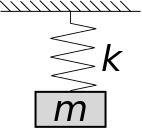
Figure 1: Sprin-mass system.
|
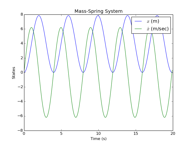
Simulating such a system with the help of SimPy is particularly simple as shown in the code section below.
from scipy.integrate import odeint from numpy import * import matplotlib.pyplot as plt def MassSpring(state,t): x = state[0] # position xd = state[1] # velocity # variables k = -5 # Nm m = 2 # kg g = 9.81 # m/s^2 # mass acceleration xdd = ((k*x)/m) + g return [xd, xdd] state0 = [0.0, 0.0] t = arange(0.0, 20.0, 0.1) state = odeint(MassSpring, state0, t) plt.plot(t, state) plt.xlabel('Time (s)') plt.ylabel('States') plt.title('Mass-Spring System') plt.legend(('$x$ (m)', '$\dot{x}$ (m/sec)')) plt.show() raw_input() |
|
The aforementioned system is particularly simple as it is expressed using linear ODEs. A slightly more difficult case arises, when one has to deal with nonlinear systems. Take for example the case of the Lorenz Attractor, a well known nonlinear system actively used to illustrate concepts of the chaos theory. Its state equations are:
The parameters σ,ρ,β are dominating the response of the system and if ones sets them as:
Then the system exhibits chaotic behavior as shown in the simulation case study below.
from scipy.integrate import odeint from numpy import * import matplotlib.pyplot as plt from mpl_toolkits.mplot3d import Axes3D def Lorenz(state,t): x = state[0] y = state[1] z = state[2] # set the constants sigma = 10.0 rho = 28.0 beta = 8.0/3.0 xd = sigma * (y-x) yd = (rho-z)*x - y zd = x*y - beta*z return [xd, yd, zd] state0 = [2.0, 3.0, 4.0] t = arange(0.0, 30.0, 0.01) state = odeint(Lorenz, state0, t) fig = plt.figure() ax = fig.gca(projection='3D') ax.plot(state[:,0],state[:,1],state[:,2]) ax.set_xlabel('x') ax.set_ylabel('y') ax.set_zlabel('z') fig.show() raw_input() |
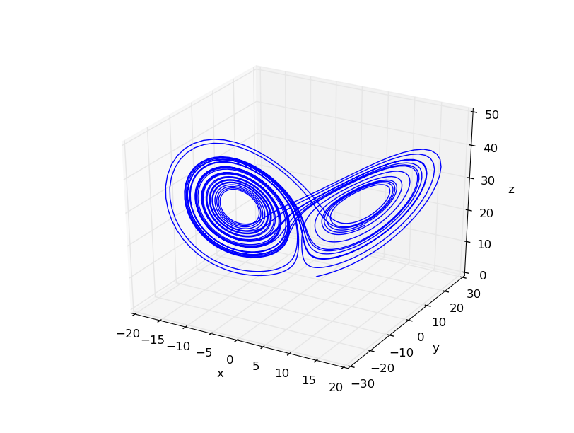
Figure 3: Lorenz Attractor expression chaotic behavior.
|
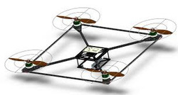
Simulation of a Quadrotor Aerial Robot
|
The classes/methods below implement the simulation of the vehicle dynamics of a quadrotor aerial robot. The system is considered to be captured using rigid body modeling and the four thrust vectors attached to it, while its self-response is only characterized by its mass and the cross-inertia terms. Within that framework, scipy is employed for the forward integration purposes of the state update, while direct calculations and linear algebra are employed for the moment/forces calculations as well as the coordinate system transformations.
|
|
File: main.py
from quadrotor_sims_params import *

if __name__ == "__main__":
    fly_quadrotor()
File: quadrotor_sims_params.py
#       __QUADROTORSIMSPARAMS__
#       This file implements the sim parameters
#       simple quadrotor simulation tool
#
#       Largely based on the work of https://github.com/nikhilkalige

from quadrotor_dynamics import QuadrotorDynamics
import numpy as np
import random
import time
import matplotlib.pyplot as plt

TURNS = 3

class SimulationParams(object):
    def __init__(self):
        self.mass = 1
        self.Ixx = 0.0053
        self.length = 0.2
        self.Bup = 21.58
        self.Bdown = 3.92
        self.Cpmax = np.pi * 1800/180
        self.Cn = TURNS
        self.gravity = 9.81

    def get_acceleration(self, p0, p3):
        ap = {
            'acc': (-self.mass * self.length * (self.Bup - p0) / (4 * self.Ixx)),
            'start': (self.mass * self.length * (self.Bup - self.Bdown) / (4 * self.Ixx)),
            'coast': 0,
            'stop': (-self.mass * self.length * (self.Bup - self.Bdown) / (4 * self.Ixx)),
            'recover': (self.mass * self.length * (self.Bup - p3) / (4 * self.Ixx)),
        }
        return ap

    def get_initial_parameters(self):
        p0 = p3 = 0.9 * self.Bup
        p1 = p4 = 0.1
        acc_start = self.get_acceleration(p0, p3)['start']
        p2 = (2 * np.pi * self.Cn / self.Cpmax) - (self.Cpmax / acc_start)
        return [p0, p1, p2, p3, p4]

    def get_sections(self, parameters):
        sections = np.zeros(5, dtype='object')
        [p0, p1, p2, p3, p4] = parameters

        ap = self.get_acceleration(p0, p3)

        T2 = (self.Cpmax - p1 * ap['acc']) / ap['start']
        T4 = -(self.Cpmax + p4 * ap['recover']) / ap['stop']

        aq = 0
        ar = 0

        sections[0] = (self.mass * p0, [ap['acc'], aq, ar], p1)

        temp = self.mass * self.Bup - 2 * abs(ap['start']) * self.Ixx / self.length
        sections[1] = (temp, [ap['start'], aq, ar], T2)

        sections[2] = (self.mass * self.Bdown, [ap['coast'], aq, ar], p2)

        temp = self.mass * self.Bup - 2 * abs(ap['stop']) * self.Ixx / self.length
        sections[3] = (temp, [ap['stop'], aq, ar], T4)

        sections[4] = (self.mass * p3, [ap['recover'], aq, ar], p4)
        return sections

def fly_quadrotor(params=None):
    gen = SimulationParams()
    quadrotor = QuadrotorDynamics()
    if not params:
        params = gen.get_initial_parameters()
    sections = gen.get_sections(params)
    state = quadrotor.update_state(sections)
    plt.plot(state)
    plt.show()
    raw_input()
File: quadrotor_dynamics.py
#       __QUADROTORDYNAMICS__
#       This file implements the dynamics of a
#       simple quadrotor micro aerial vehicle
#
#       Largely based on the work of https://github.com/nikhilkalige

import numpy as np
from scipy.integrate import odeint

class QuadrotorDynamics(object):

    def __init__(self, save_state=True, config={}):
        """
        Quadrotor Dynamics Parameters
        ----------
        save_state: Boolean
            Decides whether the state of the system should be saved
            and returned at the end
        """
        self.config = {
            # Define constants
            'gravity': 9.81,  # Earth gravity [m s^-2]
            # Define Vehicle Parameters
            'mass': 1,  # Mass [kg]
            'length': 0.2,  # Arm length [m]
            # Cross-Intertia [Ixx, Iyy, Izz]
            'inertia': np.array([0.0053, 0.0053, 0.0086]),  # [kg m^2]
            'thrustToDrag': 0.018  # thrust to drag constant [m]
        }

        self.save_state = save_state
        self._dt = 0.005  # Simulation Step
        self.config.update(config)
        self.initialize_state()

    def initialize_state(self):
        self.state = {
            # Position [x, y, z] of the quadrotor in inertial frame
            'position': np.zeros(3),
            # Velocity [dx/dt, dy/dt, dz/dt] of the quadrotor in inertial frame
            'velocity': np.zeros(3),
            # Euler angles [phi, theta, psi]
            'orientation': np.zeros(3),
            # Angular velocity [p, q, r]
            'ang_velocity': np.zeros(3)
        }

    def motor_thrust(self, moments, total_thrust):
        """Compute Motor Thrusts

        Parameters
        ----------
        moments : numpy.array
            [Mp, Mq, Mr] moments
        total_thrust : float
            The total thrust generated by all motors

        Returns
        -------
        numpy.array
            The thrust generated by each motor [T1, T2, T3, T4]
        """
        [Mp, Mq, Mr] = moments
        thrust = np.zeros(4)
        tmp1add = total_thrust + Mr / self.config['thrustToDrag']
        tmp1sub = total_thrust - Mr / self.config['thrustToDrag']

        tmp2p = 2 * Mp / self.config['length']
        tmp2q = 2 * Mq / self.config['length']

        thrust[0] = tmp1add - tmp2q
        thrust[1] = tmp1sub + tmp2p
        thrust[2] = tmp1add + tmp2q
        thrust[3] = tmp1sub - tmp2p

        return thrust / 4.0

    def dt_eulerangles_to_angular_velocity(self, dtEuler, EulerAngles):
        """Euler angles derivatives TO angular velocities
        dtEuler = np.array([dphi/dt, dtheta/dt, dpsi/dt])
        """
        return np.dot(self.angular_rotation_matrix(EulerAngles), dtEuler)

    def acceleration(self, thrusts, EulerAngles):
        """Compute the acceleration in inertial reference frame
        thrust = np.array([Motor1, .... Motor4])
        """
        force_z_body = np.sum(thrusts) / self.config['mass']
        rotation_matrix = self.rotation_matrix(EulerAngles)
        # print rotation_matrix
        force_body = np.array([0, 0, force_z_body])
        return np.dot(rotation_matrix, force_body) - np.array([0, 0, self.config['gravity']])

    def angular_acceleration(self, omega, thrust):
        """Compute the angular acceleration in body frame
        omega = angular velocity :- np.array([p, q, r])
        """
        [t1, t2, t3, t4] = thrust
        thrust_matrix = np.array([self.config['length'] * (t2 - t4),
                                  self.config['length'] * (t3 - t1),
                                  self.config['thrustToDrag'] * (t1 - t2 + t3 - t4)])

        inverse_inertia = np.linalg.inv(self.inertia_matrix)
        p1 = np.dot(inverse_inertia, thrust_matrix)
        p2 = np.dot(inverse_inertia, omega)
        p3 = np.dot(self.inertia_matrix, omega)
        cross = np.cross(p2, p3)
        return p1 - cross

    def angular_velocity_to_dt_eulerangles(self, omega, EulerAngles):
        """Angular Velocity TO Euler Angles
        omega = angular velocity :- np.array([p, q, r])
        """
        rotation_matrix = np.linalg.inv(self.angular_rotation_matrix(EulerAngles))
        return np.dot(rotation_matrix, omega)

    def moments(self, ref_acc, angular_vel):
        """Compute the moments

        Parameters
        ----------
        ref_acc : numpy.array
            The desired angular acceleration that the system should achieve. This
            should be of form [dp/dt, dq/dt, dr/dt]
        angular_vel : numpy.array
            The current angular velocity of the system. This
            should be of form [p, q, r]

        Returns
        -------
        numpy.array
            The desired moments of the system
        """
        inverse_inertia = np.linalg.inv(self.inertia_matrix)
        p1 = np.dot(inverse_inertia, angular_vel)
        p2 = np.dot(self.inertia_matrix, angular_vel)
        cross = np.cross(p1, p2)
        value = ref_acc + cross
        return np.dot(self.inertia_matrix, value)

    def angular_rotation_matrix(self, EulerAngles):
        """Rotation matix for Angular Velocity <-> Euler Angles Conversion
        Use inverse of the matrix to convert from angular velocity to euler rates
        """
        [phi, theta, psi] = EulerAngles
        cphi = np.cos(phi)
        sphi = np.sin(phi)
        cthe = np.cos(theta)
        sthe = np.sin(theta)
        cpsi = np.cos(psi)
        spsi = np.sin(psi)
        RotMatAngV = np.array([ [1, 0,            -sthe],
                                [0, cphi,  cthe * sphi],
                                [0, -spsi, cthe * cphi]
                                ])
        return RotMatAngV

    def rotation_matrix(self, EulerAngles):
        [phi, theta, psi] = EulerAngles
        cphi = np.cos(phi)
        sphi = np.sin(phi)
        cthe = np.cos(theta)
        sthe = np.sin(theta)
        cpsi = np.cos(psi)
        spsi = np.sin(psi)

        RotMat = np.array([[cthe * cpsi, sphi * sthe * cpsi - cphi * spsi, cphi * sthe * cpsi + sphi * spsi],
                      [cthe * spsi, sphi * sthe * spsi + cphi * cpsi, cphi * sthe * spsi - sphi * cpsi],
                      [-sthe,       cthe * sphi,                      cthe * cphi]])
        return RotMat

    @property
    def inertia_matrix(self):
        return np.diag(self.config['inertia'])

    def update_state(self, piecewise_args):
        """Run the state update equations for self._dt seconds
        Update the current state of the system. It runs the model and updates
        its state to self._dt seconds.

        Parameters
        ----------
        piecewise_args : array
            It contains the parameters that are needed to run each section
            of the flight. It is an array of tuples.
            [(ct1, da1, t1), (ct2, da2, t2), ..., (ctn, dan, tn)]

            ct : float
                The collective thrust generated by all motors
            da : numpy.array
                The desired angular acceleration that the system should achieve.
                This should be of form [dp/dt, dq/dt, dr/dt]
            t: float
                Time for which this section should run and should be atleast twice
                self._dt
        """
        if self.save_state:
            overall_time = 0
            for section in piecewise_args:
                overall_time += section[2]

            overall_length = len(np.arange(0, overall_time, self._dt)) - (len(piecewise_args) - 1)
            # Allocate space for storing state of all sections
            final_state = np.zeros([overall_length + 100, 12])
        else:
            final_state = []

        # Create variable to maintain state between integration steps
        self._euler_dot = np.zeros(3)
        index = 0

        for section in piecewise_args:
            (total_thrust, desired_angular_acc, t) = section
            if t < (2 * self._dt):
                continue

            ts = np.arange(0, t, self._dt)
            state = np.concatenate((self.state['position'], self.state['velocity'],
                                    self.state['orientation'], self.state['ang_velocity']))
            output = odeint(self._integrator, state, ts, args=(total_thrust, desired_angular_acc))
            output_length = len(output)
            # State update
            [self.state['position'], self.state['velocity'],
             self.state['orientation'], self.state['ang_velocity']] = np.split(output[output_length - 1], 4)

            if self.save_state:
                # Final state update
                final_state[index:(index + output_length)] = output
                index = index + output_length - 1

        return final_state

    def _integrator(self, state, t, total_thrust, desired_angular_acc):
        """Callback function for scipy.integrate.odeint.
            At this point scipy is used to execute the forward integration

        Parameters
        ----------
        state : numpy.array
            System State: [x, y, z, xdot, ydot, zdot, phi, theta, psi, p, q, r]
        t : float
            Time

        Returns
        -------
        numpy.array
            Rates of the input state:
            [xdot, ydot, zdot, xddot, yddot, zddot, phidot, thetadot, psidot, pdot, qdot, rdot]
        """
        # Position inertial frame [x, y, z]
        pos = state[:3]
        # Velocity inertial frame [x, y, z]
        velocity = state[3:6]
        euler = state[6:9]
        # Angular velocity omega = [p, q, r]
        omega = state[9:12]

        # Derivative of euler angles [dphi/dt, dtheta/dt, dpsi/dt]
        euler_dot = self._euler_dot

        # omega = self.dt_eulerangles_to_angular_velocity(euler_dot, euler)
        moments = self.moments(desired_angular_acc, omega)
        thrusts = self.motor_thrust(moments, total_thrust)
        # Acceleration in inertial frame
        acc = self.acceleration(thrusts, euler)

        omega_dot = self.angular_acceleration(omega, thrusts)
        euler_dot = self.angular_velocity_to_dt_eulerangles(omega, euler)
        self._euler_dot = euler_dot
        # [velocity : acc : euler_dot : omega_dot]
        # print 'Vel', velocity
        # print 'Acc', acc
        # print 'Euler dot', euler_dot
        # print 'omdega dot', omega_dot
        return np.concatenate((velocity, acc, euler_dot, omega_dot))